Reinforcement Learning
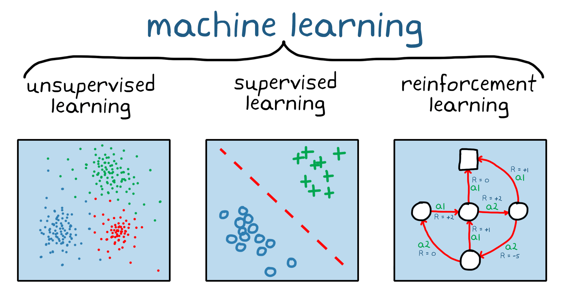
Reinforcement learning is one of the three main branches of machine learning. It’s useful when we don’t have a clear label that we want our model to predict. Instead, we have a reward—a signal that indicates how good or bad the results of a particular action were. For example, winning a game or making a profit is good; making a bigger profit is better; and crashing a Tesla is bad.
Applications
RL is typically applied in cases where sequential decisions have to be made over time, where those decisions affect future states and rewards, where labeled examples come at a significant cost, or where defining a scoring function is difficult.
- Robotics
- Autonomous vehicles
- Games
- Finance
- Alignment in LLMs (RLHF)
RL in games
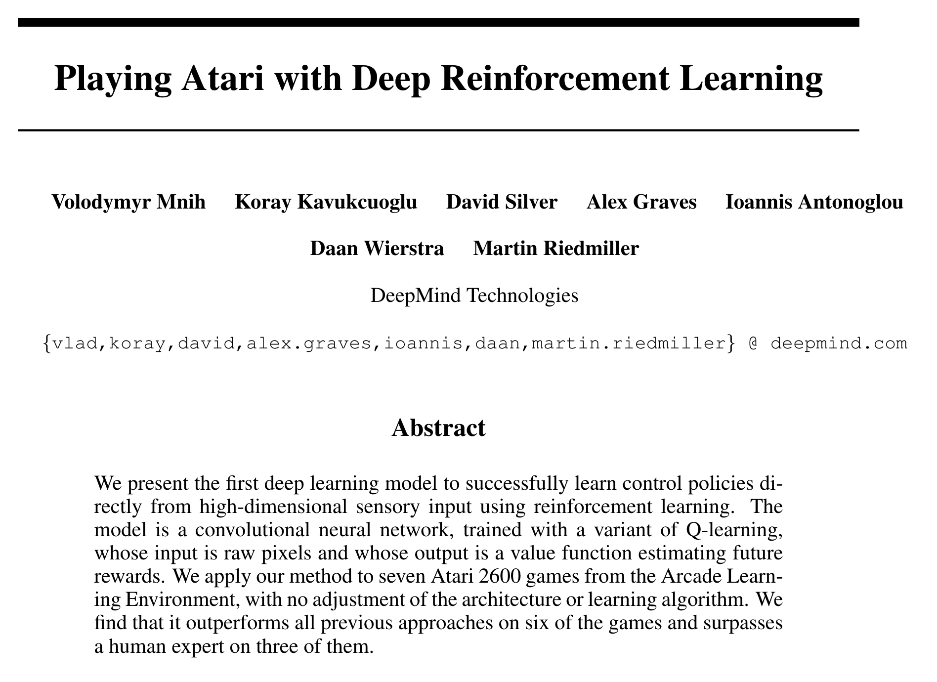
RL has seen success in games, for example AlphaGo’s victory over the world champion Go player, Lee Sedol. Researchers at DeepMind applied RL to beating Atari games.
Check out Andrej Karpathy’s post Deep Reinforcement Learning: Pong from Pixels.
RLHF
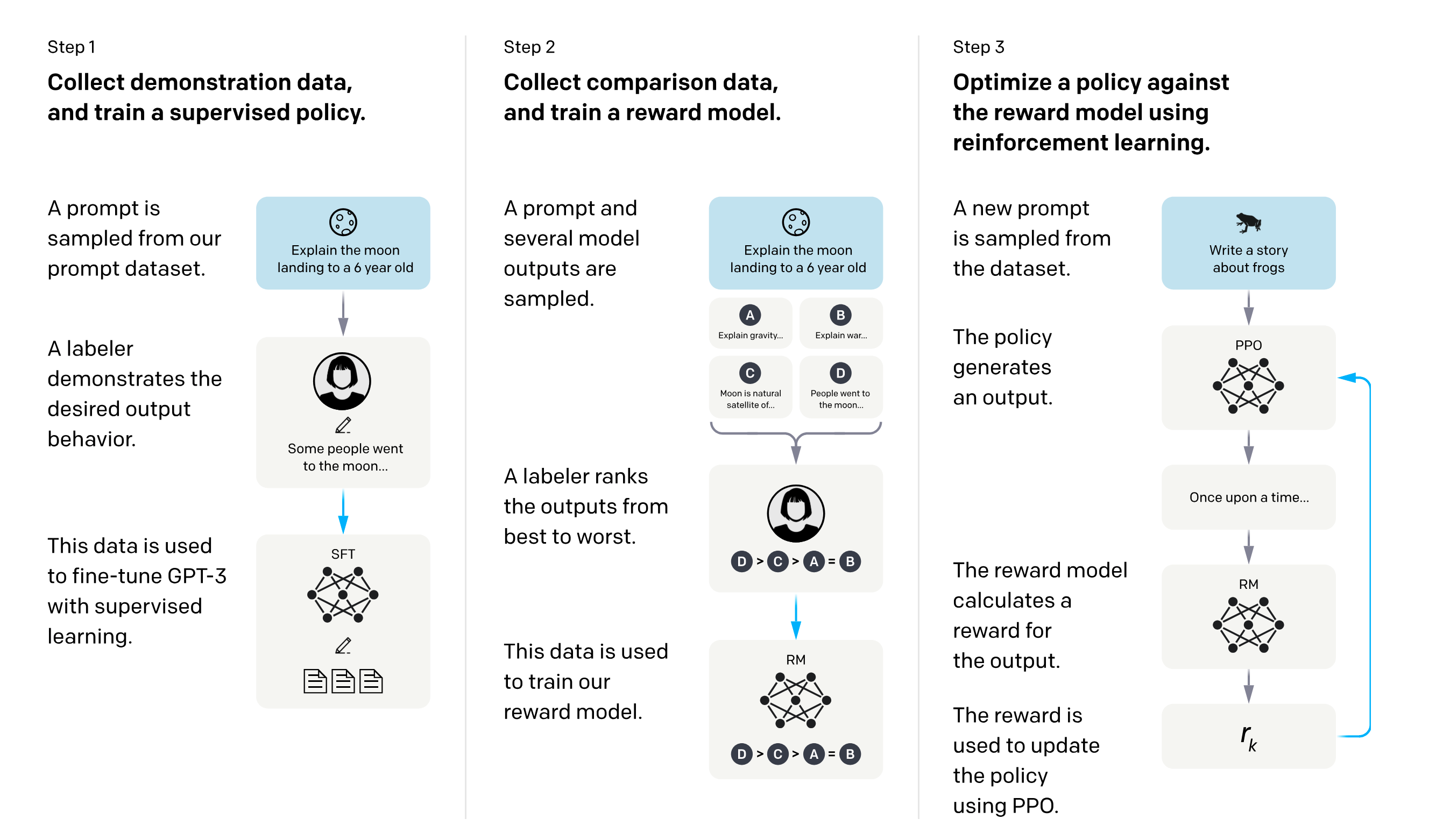
Recent success using reinforcement learning with human feedback (RLHF) to train large language models has renewed interest in RL. The diagram below from Training language models to follow instructions with human feedback (Ouyang et al, 2022) shows the training process for ChatGPT. Step 1 is supervised fine-tuning. Steps 2 and 3 are RLHF, first training a reward model on human preferences, then applying that reward model to modify the scoring of output generated by the LLM.
The insight is that it’s much easier for a human labeler to rank outputs than to produce a high-quality piece of training data. The ranking becomes the reward that helps the LLM learn to prefer the higher quality examples from the very mixed bag used during pretraining - giant text dumps of the whole internet.
The RL problem
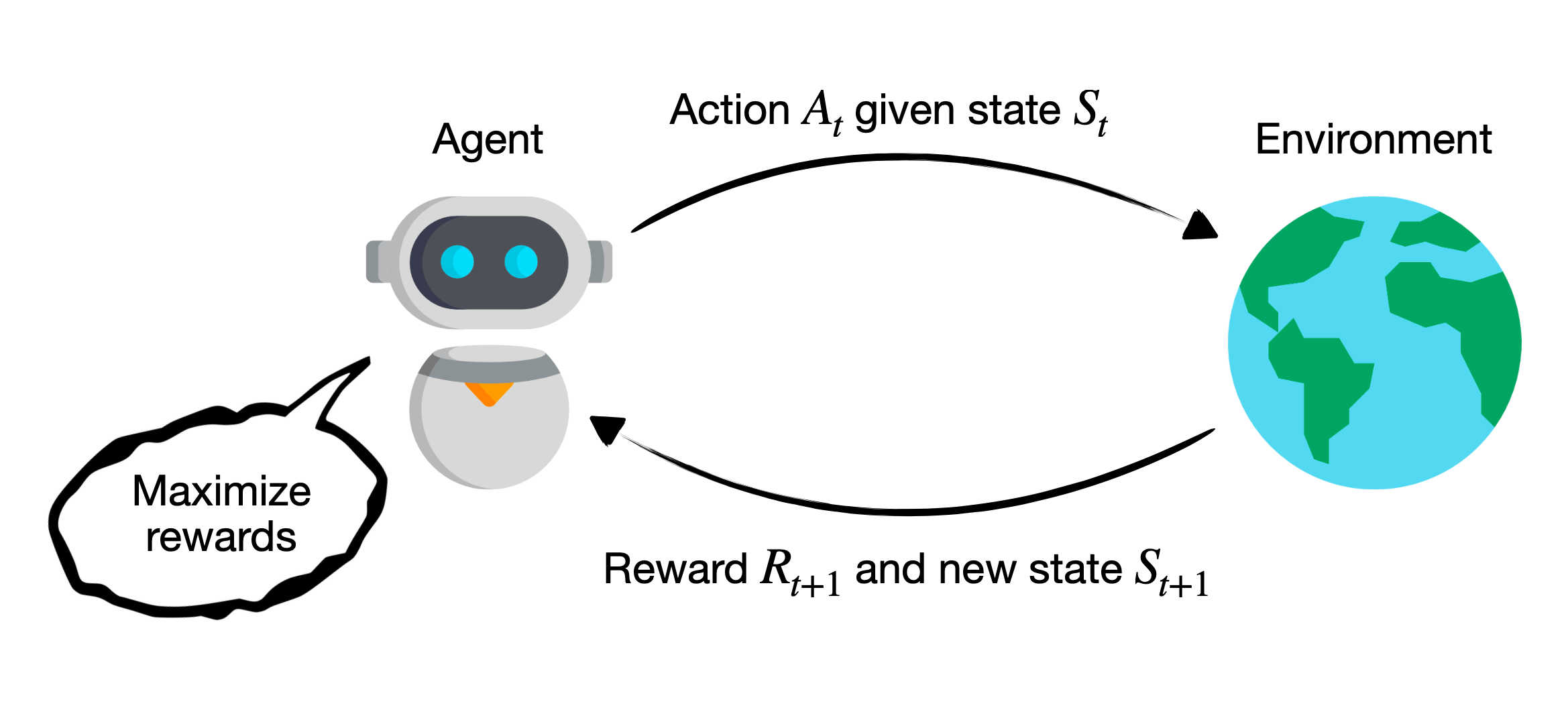
Reinforcement learning aims to “capture the most important aspects of the real problem facing a learning agent interacting over time with its environment to achieve a goal.” (Sutton and Barto) It’s a problem definition doesn’t assume a particular method for solution. Using neural networks to solve RL problems, as shown in the pong example above, is one method but not the only one.
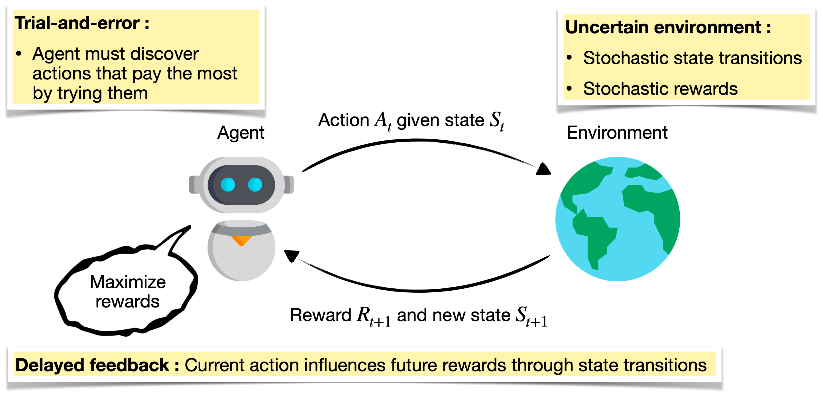
The basic elements are state, action, and reward. The agent’s goal is to choose the actions, given its observations of state, that maximize cumulative future reward.
Adding complexity
But, it gets worse. Consider the uncertainty and incomplete information with which we contend when trying to understand the world. We typically can’t observe the complete state of the world and what we can observe is subject to misinterpretation. Was that a gunshot or just fireworks? Our actions may not have the hoped-for results and we suffer the consequences if we choose unwisely. Rewards may come at a delay, long after a critical action was taken.
If we assume the environment is unchanging, we can learn an optimal policy - the mapping between state and the next action - and sit back and collect rewards. But what if the dynamics of the environment change over time? Or if competing agents adapt their strategy to counter ours? The goal of continual learning is for the agent to adapt to non-stationary environments without forgetting previously learned tasks.
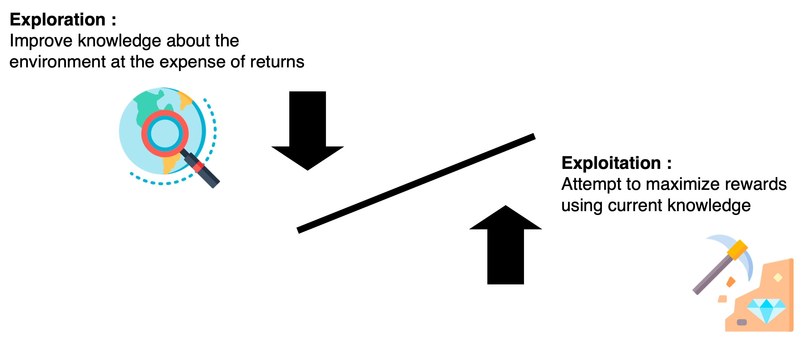
Explore/Exploit tradeoff
One important aspect of RL is the trade-off between exploration and exploitation. Exploration has a price.
“To obtain a lot of reward, a reinforcement learning agent must prefer actions that it has tried in the past and found to be e↵ective in producing reward. But to discover such actions, it has to try actions that it has not selected before. The agent has to exploit what it has already experienced in order to obtain reward, but it also has to explore in order to make better action selections in the future. The dilemma is that neither exploration nor exploitation can be pursued exclusively without failing at the task. The agent must try a variety of actions and progressively favor those that appear to be best. On a stochastic task, each action must be tried many times to gain a reliable estimate of its expected reward. The exploration–exploitation dilemma has been intensively studied by mathematicians for many decades, yet remains unresolved.” (Sutton and Barto)
Terminology and definitions
- \(\mathcal{S}\) is a finite set of states
- \(\mathcal{A}\) is a finite set of actions
- \(\mathcal{P}\) is the state transition probability matrix
- \(\mathcal{R}(s, s', a) \in \mathbb{R}\) is the immediate reward after going from state \(s\) to state \(s'\) with action \(a\).
- \(\gamma \in [0, 1]\) is the discount factor
History: The sequence of states, actions, and rewards that the agent has experienced up to time \(t\).
\[H_t = A_1, S_1, R_1, \ldots, A_t, S_t, R_t\]Current state is a function of History:
\[S_t = f(H_t)\]The Markov property: The future is independent of the past given the present.
\[P(S_{t+1} \mid S_t) = P(S_{t+1} \mid S_1, S_2, \ldots, S_t)\]Question: If the state is a function of history, why don’t we state the Markov property as:
\[P(S_{t+1} \mid S_t) = P(S_{t+1} \mid H_t)\]Markov Decision Process (MDP)
An MDP is a tuple \(\langle \mathcal{S}, \mathcal{A}, \mathcal{P}, \mathcal{R}, \gamma \rangle\).
Policy
A policy \(\pi\) is a function \(\pi: S \rightarrow A\) that tells us what action to do in a given state. It’s a mapping from states to actions.
\[\pi(A_t = a \mid S_t = s)\] \[\forall A_t \in \mathcal{A}(s), \forall S_t \in \mathcal{S}\]Value
Value is the expected return starting from state \(s\), following policy \(\pi\).
\[V^\pi(s) = E_{\pi} \{G_t \mid s_t = s\}\]…where \(G_t\) is the total discounted reward from time step \(t\):
\[G_t = R_{t+1} + \gamma R_{t+2} + \gamma^2 R_{t+3} + \ldots = \sum_{k=0}^\infty \gamma^k R_{t+k+1}\]The Bellman equation decomposes value into immediate reward and discounted value of the next state:
\[V^\pi(s) = E_\pi \{R_{t+1} + \gamma V^\pi(S_{t+1}) \mid S_t = s\}\]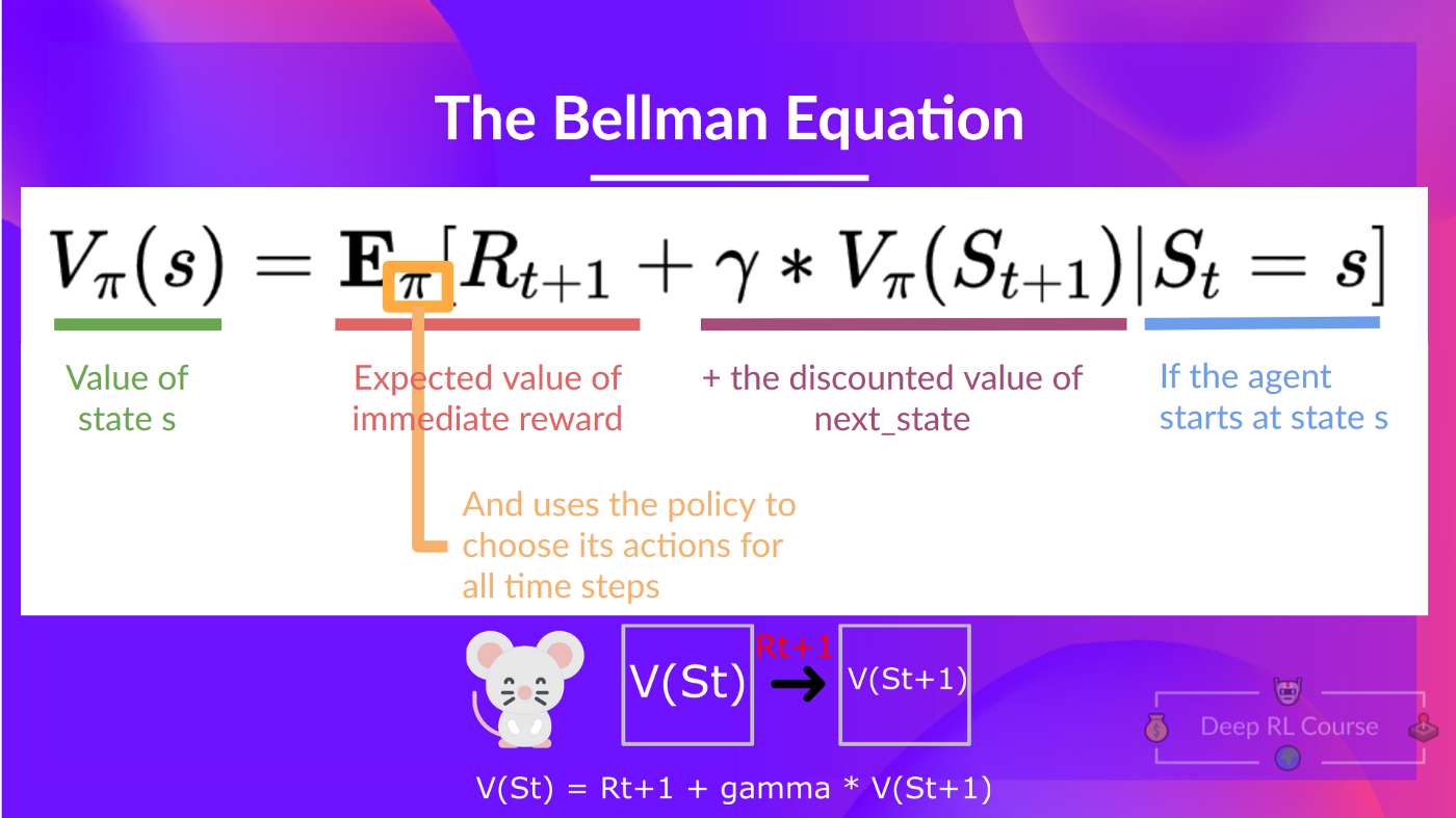
Q
\[Q: \mathcal{S} \times \mathcal{A} \to \mathbb{R}\]\(Q^\pi(s, a)\) is the “action value” function, also known as the quality function. It is the expected return starting from state \(s\), taking action \(a\), then following policy \(\pi\).
\[Q^\pi(s, a) = E_\pi \{G_t | s_t = s, a_t = a\} = E_\pi \{\sum_{k=0}^\infty \gamma^k r_{t+k+1} | s_t = s, a_t=a\}\]In Q-learning, we learn the Q function. The optimal policy then chooses that action that maximizes discounted expected returns for a given state.
Resources
- Reinforcement Learning: An Introduction by Richard Sutton and Andrew Barto
- Deep Reinforcement Learning: Pong from Pixels by Andrej Karpathy
- David Silver’s course on RL
- John Schulman Deep Reinforcement Learning and Policy Gradient Methods: Tutorial and New Frontiers
- 🤗 Deep Reinforcement Learning Course