Neural style transfer
Notes from week 4 of Convolutional Neural Networks:
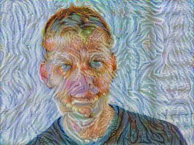
Neural style transfer takes two images and applies the style of one to the content of the other. A pretrained ConvNet is used to represent both content and style.
Content
Content is represented by the activations at some layer in the network. The content cost is then proportional to the squared difference between the content image’s activations at that layer and the generated image’s activations at that same layer.
\[J_{content}(C,G) = \frac{1}{4 \times n_H \times n_W \times n_C}\sum _{ \text{all entries}} (a^{(C)} - a^{(G)})^2\]Style
“The style matrix is also called a "Gram matrix." In linear algebra, the Gram matrix G of a set of vectors \((v_{1}, \dots ,v_{n})\) is the matrix of dot products, whose entries are \({\displaystyle G_{ij} = v_{i}^T v_{j} = np.dot(v_{i}, v_{j}) }\). In other words, \(G_{ij}\) compares how similar \(v_i\) is to \(v_j\): If they are highly similar, you would expect them to have a large dot product, and thus for \(G_{ij}\) to be large.”
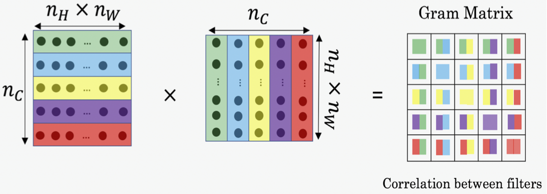
The style matrix captures information about the correlation of whatever abstract features the convolutional filters are responding to. If the generated image and the style image have similar style matrices, they’ll have similar co-occurences of these abstract features. Monet and Van Gogh seem to work well, maybe because their styles are defined by distinctive textures.
Minimizing the style cost will cause the generated image to follow the style of the style image.
\[J_{style}^{[l]}(S,G) = \frac{1}{4 \times {n_C}^2 \times (n_H \times n_W)^2} \sum _{i=1}^{n_C}\sum_{j=1}^{n_C}(G^{(S)}_{ij} - G^{(G)}_{ij})^2\]Optimization
Combining this representation from multiple hidden layers gives even better results.
\[J_{style}(S,G) = \sum_{l} \lambda^{[l]} J^{[l]}_{style}(S,G)\]Finally, we combine content and style:
\[J(G) = \alpha J_{content}(C,G) + \beta J_{style}(S,G)\]In the exercise, we initialized the generated image by adding noise to the content image. Training is done with back propagation, but instead of updating weights in the network, at each iteration we update the generated image.
References from the homework:
Harish Narayanan and Github user “log0” also have highly readable write-ups from which we drew inspiration. The pre-trained network used in this implementation is a VGG network, which is due to Simonyan and Zisserman (2015). Pre-trained weights were from the work of the MathConvNet team.
- Leon A. Gatys, Alexander S. Ecker, Matthias Bethge, (2015). A Neural Algorithm of Artistic Style
- Harish Narayanan, Convolutional neural networks for artistic style transfer.
- Github user “log0”, TensorFlow Implementation of A Neural Algorithm of Artistic Style.
- Karen Simonyan and Andrew Zisserman (2015). Very deep convolutional networks for large-scale image recognition
- MatConvNet